Field Activity #3: Conducting a Distance Azimuth Survey

Introduction

In this weeks lab adventure we will be conducting field research with less technology than one would normally prefer too.  Far too often situations come up in the field which leave you to improvise your methods.  The window can be short for data collection in the field, so going back to get the appropriate equipment may not be always feasible.  Our instructor Dr. Hupy explained how he had traveled to a foreign country and had his high end GPS unit seized at customs.  In this type of situation you can't just run back to the office and grab another one, so you need to be prepared to improvise.  Dr. Hupy's example is just one of a multitude of possibilities which could happen to someone doing field research.  Knowing how to collect the location data accurately in improvised situations is the focus of this lab exercise.

Methods

To start this exercise Dr. Hupy took our entire class outside to give us a demo of how to use the equipment and to make sure we had the data recorded in the proper format for importing into ArcMap.  He had also randomly put us into groups of 2 to work with for the remainder of this field activity.  My partner was Casey Aumann. (Casey's Blog)

Our class was given instruction on how to use the TruPulse 360.  The TruPulse 360 is a laser range finder.  The TruPulse 360 also has the capability of telling you the azimuthal direction you are facing in degrees.  You are able to locate the image in the view finder and fire the laser with the button on the top of the unit.  If you want to see what your azimuthal direction is you must use one of the two buttons on the side to toggle through the selection until AZ is displayed in the view finder.  The unit has multiple settings for distance.  Our class was instructed to use the SD (Slope Distance) setting on the unit.

(Fig. 1)  The TruPulse 360 is on the left and the picture on the right is an example of the view withing the viewfinder

After recording just a handful of points we returned to the computer lab to input our points we had recorded into Excel and then import the table of points into ArcMap creating a feature class.  Upon adding the feature class to the data frame, and a base map to the background we noticed something was askew.  The point of origin was off and direction of the lines was off enough to visibly notice at a quick glance.  At the end of the class period, our class and Dr. Hupy were unable to resolve the issue.  Assuming the calibration was off, the following day Dr. Hupy went out with the TruPulse 200 and attempted to recalibrate the unit.  He went to the same location as our class did the day before, with terrible results.  Dr. Hupy had couple reoccurring problems including, failure to calibrate, or the compass would point to a different north direction each time.  After all the trouble, Dr. Hupy relocated to a wooded area and was able to calibrate the unit with no issues.  Dr. Hupy believes there was electrical interference somewhere on the corner of the building or underground which was causing all of the incorrect readings.  Using this information my partner and I chose to survey a different location on campus.

(Fig. 2) This is the results of the trail run with Dr. Hupy.  The red dot is actually where they points were taken from and the pink dots are where the green lines should line up too.  Not all the pink dots can be see on this extent of the photo.

For this exercise Casey and I used the TruPulse 360 unit to obtain our distance and azimuth information.  Additionally, we used my personal Garmin 62s to obtain our point of origin.  On the afternoon Wednesday September 30th, 2015 my partner and I headed to the the campus courtyard on the University Wisconsin Eau Claire Campus.  The decision to use the courtyard was due to a plethora of large stone benches, light posts and other features for us to measure.  The area wide open though it does fall between a lot of buildings, we were hoping to reduce the chance of being hampered by electrical interference.

When we arrived at the courtyard we picked a location in the center of the courtyard with a view of all the features to be surveyed.  The location we chose was on a paved surface which had individual squares.  We picked a square to stand in and record our point of origin.  Having this square helped us to make sure we remained in the exact same location as we recorded our data.

(Fig. 3) My lab partner standing in the square we chose to record our data from.

For this lab exercise we had to record the distance, azimuth, and object attribute for at least 100 different points in our study area.  As suggested by Dr. Hupy we double check our angles and make sure we weren't getting any interference using a compass.  Everything appeared to be in check so we proceeded to collect our data.  In the courtyard there are just over 50 stone benches, so we decided to use them as our first features to measure.  It was a beautiful afternoon so there was a number of people utilizing the courtyard and the benches.  This made it difficult to obtain a accurate reading from some of the benches as people were sitting or leaning up against them.  We were standing in a lower spot of the courtyard, which limited the view of some benches.  With only a small portion of the bench visible it was tough to get an accurate reading, especially if it was any distance away.  The TruLaser has a 7x magnification which increases any movement or shaking in the view finder adding to the toughness of locking on to small object for an accurate reading.

We directly entered the data in to an Excel file using a laptop to eliminate a step of having to transfer the data later if we were to record the data on paper.  Having done a trial run in class a few days before we already knew what the format had to be to achieve the correct results.

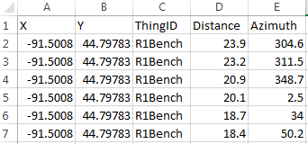(Fig. 4) The formatting used to record the data in Excel.

After recording the data all of the benches, we decided the light poles within the courtyard would be our next feature to collect data from.  The light poles are not very large in diameter, so getting an accurate reading from them each time posed to be a challenge.  We focused in on the head of the lamp which was considerably larger in diameter than the post itself.  After collecting and recording all of the light pole information, we choose to survey the larger trees and ground signs around the courtyard.  When completed we ended up with 107 points we collected data for.

Before we could covert the data to a feature class in ArcMap we needed to take the point of origin from the GPS and convert it from degrees, minuets, seconds to decimal degrees.  Dividing the minuets by 60 gave us the decimal we needed to accurately display our point of origin.

With all the data in the Excel file I imported the table into ArcCatalog.  The next step was to open new blank file in ArcMap.  To display our data, I had to run a tool called Bearing Distance To Line using the table I had imported as the input data.  The tool is located under Data Management Tools and then under Features in ArcToolBox.  Using the data within the table the tool plotted the distances as lines from the point of origin at the given angle on the map surface.  See figure 4 for the results from this tool.

(Fig. 5)  The result after running the Bearing Distance To Line tool.

(Fig. 6)  Illustration of how the bearing distance to line tool works in ArcMap.

Once I had utilized the bearing distance to line tool, I was able to convert end of the line opposite the point of origin to a point using the Feature Vertices to Points tool with in ArcMap.  This tool is found in the same Features folder as the Bearing Distance to Line tool.  Giving the end of the line and endpoint helps you visualize the end of the line and also give the feature a determinable location on the map.

(Fig. 7)  The result of running the Feature Vertices to Points tool.

Once both of the above tools had been run I loaded in a base map of the study area in to ArcMap.  The basemap will allow me to overlay my feature classes I created to determine how accurate our data collection was and produce a map with my results.  I was unable to use the standard basemap available from ArcMap as my study area was built/created after the basemap photo was taken.Using data available to me through the university, I loaded a raster image from the City of Eau Claire file that contained my study area.  Since the basemap was projected into a Eau Claire County specific projection, I projected both my lines and endpoint feature classes to the same projection to give me the best results.  My final step was to complete the metadata.

(Fig. 8)  The finished map of our study area in the courtyard of UWEC campus.

(Fig. 9) Metadata completed.

Discussion

This lab provided good exposure to collecting data and issues which arise in the field while collecting data.  The purpose of the lab was to expose us to a "basic" survey technique which we could use in the field should our "high end" equipment fail us for one reason or another.  I realize everything is relative, however the TruLaser 360 we were using costs in the neighborhood of $1,500+ dollars.  Now I understand this is no where near the most expensive surveying tool on the market but it costs enough that not everyone is going to be carrying one around in their pocket as a "backup".  I feel that a compass and long tape reel is probably more "basic".  Knowing this tool exists now I would definitely add it to the list of tools which would be handy in conducting field surveying, especially if you are working alone.

With all technology comes limitations.  The example of the electromagnetic interference we experienced is a prime example.  Looking at my final map I believe we experienced some issues with the technology we used.  Our point of origin is off by a couple feet.  This could be caused by a number of issues.  It is possible we had more interference affecting the location.  Also, the accuracy range of a personal GPS is at best +- 3 meters.  Secondly, the point angles are off of their actual location.  This is partially due to the origin point being off but that is not the complete answer.  It is my feeling we had electromagnetic interference play games with us.  The points on the West side of the point of origin are off more than the points on the East side of the map.  I have no plausible explanation for this at the moment.

The collection of the data went smoothly.  I used the TruLaser 360 to collect all of the data numbers for all of the benches so we would have less chance of being confused as to which ones had already been done.  Also, given the benches were in row form, we decided to work from right to left and finish the complete row before moving on to the next one.  We implemented the same processes for the other features, except I was entering the data into the Excel file while my partner collected the data.

Conclusion

This lab activity proved to be very educational in many different areas.  Learning this new method of locating and plotting points will be very beneficial in the future should technology let me down as I know it will. Using a survey tape measure and compass as discussed before would be a good way to double check the accuracy of your equipment.  The introduction to the TruLaser is now another tool I am familiar with and can put to use if available.  Continued use of Excel and importing tables into ArcMap is a great way to understand and see the proper way to format data to assure it will be displayed correctly the first time.